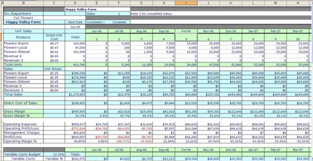
On a Google Spreadsheet, you are allowed to freeze up to 10 rows and up to 5 columns. When you freeze these cells, you will be able to see them wherever you go on the spreadsheet. This is especially useful when the frozen cells are headers. This way, you will not lose track of where you are inputting your data. To freeze cells on a Google Spreadsheet, proceed to step 1.
Steps
Launch your browser.
To get started, open your preferred web browser (Internet Explorer, Mozilla Firefox, Google Chrome, etc.) by tapping on its icon on your desktop, and go to drive.google.com.
Log in.
If you are not already logged in, Google Drive will ask you to sign in with your Google account information. If your account name is already indicated on the page, just enter your password; otherwise, type in your username and password on the fields provided.
Open a spreadsheet file.
You can either open an existing file or create a new one. The spreadsheet file will open on a new tab of your browser.
- If you have an existing spreadsheet file, locate and click on the file name in the file list at the middle of the screen.
- If you are going to create a file, click the “Create” button on the top-left corner and click on “Spreadsheet.”
Access the View menu.
Click “View” at menu bar of the spreadsheet to bring down the View menu.
Point your mouse over the option you want.
You can either freeze rows or freeze columns; whichever option you point to, a small window will pop up on the side of the View menu.
- If you want to freeze the cells at the top of the spreadsheet, point your mouse to “Freeze rows.”
- If you want to freeze the cells vertically, point to “Freeze columns.”
Select the number of columns or rows to freeze.
You can freeze up to 10 rows and 5 columns. Simply click on the number rows or columns you would like to freeze.
